

You don’t always have enough images to train a deep neural network. Here is how you can teach your model to learn quickly from a few examples.
Why do we care about Few-Shot Learning?
In 1980, Kunihiko Fukushima developed the first convolutional neural networks. Since then, thanks to increasing computing capabilities and huge efforts from the machine learning community, deep learning algorithms have never ceased to improve their performances on tasks related to computer vision. In 2015, Kaiming He and his team at Microsoft reported that their model performed better than humans at classifying images from ImageNet. At that point, one could argue that computers became better than us at harnessing billions of images to solve a specific task. Hurrah!
However, if you are not Google or Facebook, you won’t always be able to build a dataset with that many images. When you work in computer vision, you sometimes have to classify images with only one or two examples per label. At this game, humans are still to be beaten. Show a picture of an elephant to a baby and they will never fail to recognize an elephant from now on. If you do the same thing with your Resnet50, you might get disappointed by the result. This problem of learning from few examples is called few-shot learning.
For a few years now, the few-shot learning problem has drawn a lot of attention in the research community, and a lot of elegant solutions have been developed. The most popular solutions right now use meta-learning, or in three words: learning to learn. Keep reading if you want to know what it is and how it works for few-shot image classification.
The Few-Shot Image Classification task
First, we need to define the N-way K-shot image classification task. Given:
- a support set composed of N labels and, for each label, K labeled images;
- a query set composed of Q query images;
the task is to classify the query images among the N classes given the N×Kimages in the support set. When K is small (typically K<10), we talk about few-shot image classification (or one-shot in the case where K=1).
.webp?width=706&height=502&name=1%20(1).webp)
The Meta-Learning paradigm
In 1998, Thrun & Pratt stated that, given one task to solve, an algorithm is learning “if its performance at the task improves with experience”, while, given a family of tasks to solve, an algorithm is learning to learn if “its performance at each task improves with experience and with the number of tasks”. We will refer to the last one as a meta-learning algorithm. It doesn’t learn how to solve a specific task. It successively learns to solve many tasks. And each time it learns a new task, it becomes better at learning new tasks: it learns to learn.
Formally, if we want to solve a task T, the meta-learning algorithm is trained on a batch of training tasks {Tᵢ}. The training experience gained by the algorithm from its attempts at solving these tasks is used to solve the ultimate task T.
For instance, consider the task T shown in the previous figure. It consists in labeling images as Labrador, Saint-Bernard or Pug using the information from 3x2=6 labeled images of those same breeds. One training task Tᵢ could be to label images as Boxer, Labradoodle, or Rottweiler, using the information from 3x2=6 labeled images of the same breeds. The meta-training process is a succession of these tasks Tᵢ, with, each time, different breeds of dogs. We expect the meta-learning model to get better “with experience and the number of tasks”. Finally, we evaluate the model on T.
.webp?width=785&height=542&name=2%20(1).webp)
Now how do we do that? Say you want to solve the task T (with the Labrador, the Saint-Bernard and the Pug). Then you will need a meta-training dataset with a lot of dogs from a lot of different breeds. You could use for instance the Stanford Dogs Dataset, which contains more than 20k dogs extracted from ImageNet. We will call this dataset D. Note that D doesn’t need to contain any Labrador, Saint-Bernard or Pug for the process to work.
From D we sample batches of episodes (see below). Each episode corresponds to an N-way K-shot classification task Tᵢ that resembles T (typically we use the same N and K). After the model solved every episode in the batch (i.e. it labeled the images of every query set), its parameters are updated. This is usually done by backprogating the loss resulting from its classification inaccuracy on the query sets.
This way, the model learns across tasks to accurately solve a new, unseen few-shot classification task. Where a standard learning classification algorithm will learn a mapping image→label, the meta-learning algorithm typically learns a mapping support-set→c(.) where c is a mappingquery→label.
Meta-Learning algorithms
Now that we know what it means when an algorithm meta-trains, one mystery remains: how does the meta-learning model solve a few-shot classification task? Of course, there is more than one solution. Here, as authentic cool kids, we will focus on the most popular ones.
Metric Learning
The basic idea of metric learning is to learn a distance function between data points (like images). It has proven to be very useful for solving few-shot classification tasks: instead of having to fine-tune on the support set (the few labeled images), metric learning algorithms classify query images by comparing them to the labeled images.
.webp?width=608&height=521&name=3%20(1).webp)
Of course, you can’t compare images pixel by pixel, so what you want to do is compare images in a relevant feature space. To be clear, let’s detail how metric learning algorithms solve a few-shot classification task (defined above as a support set of labeled examples, and a query set of images we want to classify):
- We extract embeddings from all images of the support and query set (typically with a convolutional neural network). Now each image that we have to consider in the few-shot classification task is represented by a 1-dim vector.
- Each query is classified depending on its distance to support set images. There are many possible design choices for both the distance function and the classification strategy. An example would be Euclidean distance and k-Nearest Neighbors.
- During meta-training, at the end of the episode, the parameters of the CNN are updated by backpropagating the loss resulting from the classification error on the query set (typically a cross-entropy loss).
The two reasons why several metric learning algorithms are published every year to solve few-shot image classification is that:
- they empirically work quite well;
- the only limit is your imagination. There are many ways to extract the features and even more ways to compare these features. We will now go over a few existing solutions.
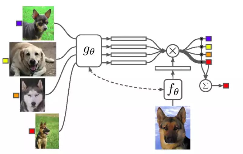
Matching Networks algorithm. The feature extractor is different for support set images (left) and query images (bottom). The query’s embedding is compared to every image in the support set using cosine similarity. It is then classified with a softmax. Figure from Vinyals et al.
Matching Networks (see above) is the first metric learning algorithm using meta-learning. In this method, we don’t extract the features in the same way for the support images and for the queries. Oriol Vinyals and his team from Google DeepMind had the idea of using LSTM networks to make all images interact during the feature extraction. They call it Full Context Embedding, because you allow the network to find the most appropriate embedding knowing not only the image to embed, but also all other images in the support set. It makes their model perform better than when all images are passed through a simple CNN, but it also needs more time and a bigger GPU.
In more recent works, we don’t compare the query images with every image in the support set. Researchers from the University of Toronto proposed Prototypical Networks. In their metric learning algorithm, after the features are extracted from the images, we compute a prototype for each class. For this, they use the mean of the embeddings of every image in the class. (But you can imagine thousands of ways to compute these embeddings. The function just needs to be differentiable, for backpropagation.) Once the prototypes are computed, the queries are classified using Euclidean distance to the prototypes (see below).
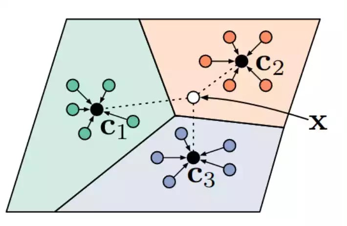
Despite its simplicity, Prototypical Networks still yield state-of-the-art results. More complex metric-learning architectures have been developed later, like a neural network to represent the distance function (instead of Euclidean distance). This slightly improves the accuracy, but I believe that to this day, the prototype idea is the idea with the best value in the field of metric learning algorithms for few-shot image classification (if you disagree, please leave an angry comment).
Model-Agnostic Meta-Learning
We will end this review with Model-Agnostic Meta-Learning (MAML), currently one of the most elegant and promising meta-learning algorithms. It’s basically Meta-Learning in its purest form, with two levels of backpropagation through the neural network.
The core idea of this algorithm is to train a neural network towards parameters that can adapt quickly and with few examples to a novel classification task. I offer you below a visualization of how MAML works on one episode of meta-training (i.e. on a few-shot classification task Tᵢsampled from D). Assume you have a neural network M parameterized with 𝚯:
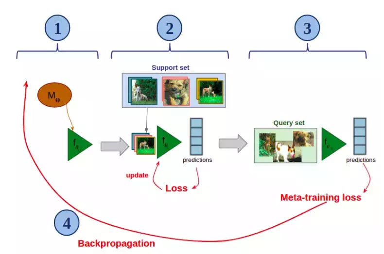
- Create a copy of M (here named f)and initialize it with 𝚯 (on the figure, 𝜽₀=𝚯).
- Quickly fine-tune f on the support set (only a few gradient descents).
- Apply the fine-tuned f on the query set.
- Backpropagate the loss resulting from the classification error through this whole process, and update 𝚯.
Then, in the next episode, we create a copy of the updated model M, we run the process on a new few-shot classification task, and so on.
During meta-training, the MAML learns initialization parameters that allow the model to adapt quickly and efficiently to a new few-shot task with new, unseen classes.
To be fair, MAML currently doesn’t work as well as metric learning algorithms on popular few-shot image classification benchmarks. It is quite hard to train because there are two levels of training, so the hyper-parameters search is much more complex. Plus, the meta-backpropagation implies the computation of gradients of gradients, so you have to use approximations to be able to train it on standard GPUs. For these reasons, you would probably rather use metric learning algorithms for your projects at home or at work.
But the reason why Model Agnostic Meta-Learning is so exciting is that it is Model Agnostic. This means that it can virtually be applied to any neural network, for any task. Mastering MAML means being able to train any neural network to adapt quickly and with few examples to a new task. Chelsea Finn and Sergey Levine, authors of the MAML, applied it to supervised few-shot classification, supervised regression and reinforcement learning. But with imagination and hard work, you can use it to transform any neural network into a Few-Shot-efficient neural network!
That’s it for this tour inside the exciting world of meta-learning. Few-Shot Learning has been dragging much attention in computer vision research recently, so the field is evolving really quickly (if you’re reading this in 2020, I suggest you look for a more recent source of information). Who knows how good neural networks will be at learning a visual concept from a single glance in the next few years?
If you are looking for Machine Learning expert's, don't hesitate to contact us !
Thanks to Antoine Toubhans, Emna Kamoun, Raphaël Meudec, Hugo Lime, Bastien Ponchon, Nicolas Jean, and Laurent Montier.